Breadth-First Search

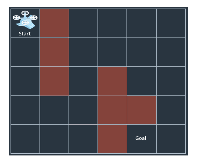
In this exercise, you'll implement breadth-first search to find a path from start to goal in a grid world like the one shown above. In this case, the grid represents your state space and the individual states that your vehicle can be in are simply positions within the grid. Using numpy in Python, you can represent this grid in the following manner:

import numpy as np
grid = np.array([
    [0, 1, 0, 0, 0, 0],
    [0, 1, 0, 0, 0, 0],
    [0, 1, 0, 1, 0, 0],
    [0, 0, 0, 1, 1, 0],
    [0, 0, 0, 1, 0, 0],
])

Within this numpy array, zeros represent the free space and ones represent obstacles. Positions within the grid are denoted just like you would in any matrix (or image) representation where (i, j) indicates row i column j, and the position (0, 0) is in the upper lefthand corner.

Python data structures for search

The search process involves keeping track of things like all your partial plans and positions visited so far. Python features a number of data structures that you could use for keeping track of actions, partial plans and visited locations, but not all data structures are created equal! Depending on your use case, different structures will perform more or less efficiently.

In this exercise, you'll keep track of which cells you can expand into, your visited list and all your partial plans using a combination of a Python queue, a set and a dictionary. The way this will work is that you'll keep track of all the cells that are possible to expand into within the queue, all the cells you've already visited in the set, and how you moved through the grid (your partial plans) in the dictionary.

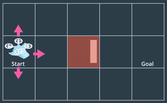
For example, using the grid world from the previous exercise, you have three possible actions from the start location:

The first step in the process is then to initialize a Queue() object and add the start location to it:

from queue import Queue
start = (1, 0) # Location in (i, j) of the start location in the image above
q = Queue()
q.put(start)

Next, initialize a set() object for your visited list and add the start location to it.

visited = set()
visited.add(start)
print(visited)
>>> {(1, 0)}

Then define an empty dictionary, where you'll record how you moved through the grid and a goal location, which in this example is (1, 4).

branch = {}
goal = (1, 4)

Next, you'll explore which actions are valid given your current position in the grid. In the first project, you used the Enum class to keep track of the state of your vehicle and here we'll use it to keep track of the action set like this:

from enum import Enum

class Action(Enum): 
    LEFT = (0, -1)
    RIGHT = (0, 1)
    UP = (-1, 0)
    DOWN = (1, 0)

    def __str__(self):
        if self == self.LEFT:
            return '<'
        elif self == self.RIGHT:
            return '>'
        elif self == self.UP:
            return '^'
        elif self == self.DOWN:
            return 'v'

Here we've defined each action as a tuple containing the indices (i, j) corresponding to how that action moves you within the grid. We've also included a string representation for each action to be used later in visualizing the path. You could do something similar with a dictionary but using an Enum object is a nice clean way of keeping track of your actions and other associated properties like, in this case, a string representation of each action.

So in the example case, valid actions are UP, DOWN and RIGHT, corresponding to movements of (-1, 0), (1, 0) and (0, 1), respectively. Or in code:

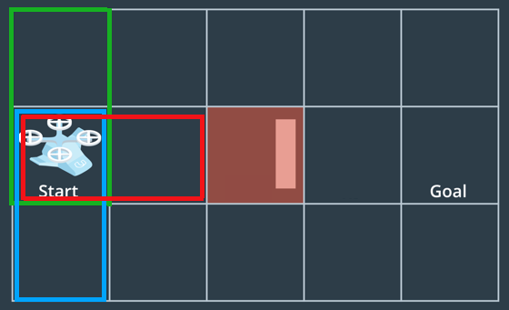
valid = [Action.UP, Action.RIGHT, Action.DOWN]

The next thing to do is expand using each of these actions:

You'll find the grid locations of these new cells one at a time based on the original cell (start in this case) and the actions that took you to get there. You'll then step through and determine whether each new cell is already on your visited list. If so, ignore it, if not, add it to the queue and visited list, and record in your branch dictionary the cell you came from and action that took you there.

current_node = start
for action in valid:
    # delta of performing the action
    da = action.value
    next_node = (current_node[0] + da[0], current_node[1] + da[1])

    # Check if the new node has been visited before.
    # If the node has not been visited you will need to
    # 1. Mark it as visited
    # 2. Add it to the queue
    # 3. Add how you got there to branch
    if next_node not in visited:                
        visited.add(next_node)               
        q.put(next_node)          
        branch[next_node] = (current_node, action) 

print(q.queue)
print(visited)
print(branch)

# And this output looks like:
>>> deque([(1, 0), (0, 0), (1, 1), (2, 0)])
>>> {(2, 0), (1, 0), (0, 0), (1, 1)}
>>> {(0, 0): ((1, 0), <Action.UP: (-1, 0)>), (1, 1): ((1, 0), <Action.RIGHT: (0, 1)>), (2, 0): ((1, 0), <Action.DOWN: (1, 0)>)}

You can employ the methods above to implement breadth-first search and when you finally arrive at the goal, it's time to retrace your steps through the branch dictionary to figure out how you got there! That looks something like this:

# Retrace your steps
path = []
n = goal
while branch[n][0] != start:
    # Append each new node to the path as you work your way back
    path.append(branch[n][1])
    n = branch[n][0]
# One last time to append the start location
path.append(branch[n][1])

# And reverse the order to make it a path from start to goal
path = path[::-1]

Breadth-first search exercise

Now it's your turn! Remember the name of the game for breadth-first search is to keep track of visited cells and all your partial plans and always expand the shortest partial plan first. Check out the notebook below and complete the TODOs in the breadth_first() function. Is your search method successful? What about if you modify the grid? Can you always find the shortest path? As an extra challenge, figure out how to convert your implementation from breadth-first search to depth-first search!

Good luck! And for a peek at our breadth-first solution, scroll to the link at the bottom of the notebook.